Hotspot Swells Revisited

Scott D. King & Claudia Adam

Department of Geosciences, Virginia Tech, Blacksburg, VA; sdk@vt.edu ; ca3@vt.edu or claudia.m.adam@gmail.com

This webpage is a summary of: King, S. D. and C. Adam (2014) Hotspot Swells Revisted, Phys. Earth Planet. Int., 235, 66-83, DOI: 10.1016/j.pepi.2014.07.006.

The initial idea behind this work was very simple; does the remarkable improvement in our knowledge of the structure of the ocean floor and access to high-resolution gridded topography/bathymetry data improve estimates of the geometry of hotspot swells? Tom Crough (1983) compiled the first global list of hotspot swells.  For the North Atlantic, he took depth anomaly calculations from Cochran & Talwani (1977) while in the Central Pacific he used data from Crough & Jarrard (1981) and Crough (1978). Thus, the data came from different sources with differing resolution. His estimate of swell heights ranged from 500-1,200 m and swell width’s ranged from 1,000-1,500 km with an estimated accuracy of roughly ±200 m.  Davies (1988) used the swell heights compiled by Crough (1983) and assumed a width of 1000 km for all hotspot swells to estimate the buoyancy necessary to dynamically maintain these swells.  Sleep (1990) expanded on the list of Davies (1988) list but was forced to guess values for a number of hotspots while for others Sleep referred back to Crough’s work. 

Could this messy situation be improved?

We created a depth anomaly map by taking a gridded topographic relief model (ETOPO2) and subtracting the theoretical depth predicted by Parsons & Sclater (1977).  We took the age of the ocean floor from Müller et al. (2008) and then corrected the bathymetry for sediment loading using Whittaker et al. (2013) (Figure 1).  We then calculated swell height and width.  One of us plotted cross-sections perpendicular to the direction of plate motion, using HS3-Nuvel1a (Gripp & Gordon, 2002) and the other used MiFil (Adam et al., 2005), a method to filter out short wavelength seamounts and volcanic construction.  Further details regarding the methodology can be found in out paper (King & Adam, 2014).

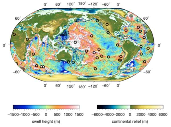
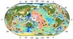
Figure 1: Global Depth Anomaly Map. In the oceans, the depth anomaly map is created by subtracting the theoretical depth predicted by Parsons & Sclater (1977) from ETOPO2 and correcting for sediment loading using Whittaker et al. (2013).   On land, topography is taken from ETOPO2.

Even with filtering techniques and much higher resolution topography/bathymetry data, the measurements of hotspot swell and width are more subjective than we realized when we first undertook the work.  We correlated the width and height measurements made using the cross-section and MiFil methods on the same depth anomaly grid and found a standard deviation of 179 km for width and 440 km for height.  Because the buoyancy flux is the product of width and height, we also correlated the product of width and height from the two methods.  The product of width and height had a standard deviation 235 km², smaller than the product of individual standard deviations.  This is because there is a tradeoff between width and height; one can often fit a swell with a greater width and lower height or a narrower width and a greater height.  Some of the difference in the measurements reflects the individual researchers choice of whether to place greater emphasis on the width or height.  If one takes the swell geometry information and calculates buoyancy flux, uncertainties are introduced by the choice of plate velocity model. For example, the difference between using HS3-Nuvel1a versus NNR in the estimate of buoyancy flux is non-negligible.  For small swells located on slow plates, it is generally larger than 60%, for larger swells it is in the order of 20%.

The largest buoyancy fluxes are found for Hawaii, Society, Macdonald, Iceland, Afar, Marquesas, Rarotonga, and Samoa.  If we apply the constraint of Abers & Christensen (1996) based on plume models that a buoyancy flux greater than 1 Mg/s is necessary for a plume from the core, then these are the only hotspots the could have a plume origin.  We wish to point out, that a swell of this magnitude does not prove a plume origin, it is simply a necessary condition, if one accepts the modeling of Abers & Christensen (1996).  Evaluating the work of Abers & Christensen (1996) was beyond the scope of this project.  We did not set out to prove or disprove the plume hypothesis.  We simply wanted to provide a new global characterization of hotspots swells.

In answer to our original question, has the remarkable improvement in our knowledge of the structure of the ocean floor improved our estimates of hotspot swells, the answer is both yes and no.  The resolution of freely available digital elevation models (e.g., ETOPO2) and age grids (Müller et al., 2008) make it easy to create depth anomaly maps of sufficiently high resolution that data coverage or resolution are not the limiting challenges. Part of the problem is that no other hotspot looks like Hawaii.  Hawaii is the largest hotspot swell and is located in an ideal setting, far from plate boundaries, continent ocean boundaries, fracture zones, etc. At Kerguelen, which is a plateau, separating the plateau and any swell contribution is highly subjective.  Some hotspots are located on the inclined continental shelf (e.g., Baja, Bowie, Cape Verde, the Canaries, Cobb and Fernando) and these are also very challenging.

We included plots of depth anomalies for each hotspot in our online supplement.  Naturally, we made many more plots in the course of our analysis, changing the map scale along with other assumptions.  However, our goal was to enable the reader to look at individual cases and make their own judgment.

References

• Albers, M. and U. Christensen (1996), The excess temperature of plumes rising from the core-mantle boundary, Geophys. Res. Lett., 23, 3567-3570.
• Adam C., V. Vidal, and A. Bonneville (2005), MiFil: A method to characterize seafloor swells with application to the south central Pacific, Geochem. Geophys. Geosyst., 6, Q01003. doi:10.1029/2004GC000814.
• Cochran, J. R, and M. Talwani (1977), Free-air gravity anomalies in the world's oceans and their relationship to residual elev­ation, Geophys. J. R. Astron. Soc., 50, 495- 552.
• Crough, S. T. (1983), Hotspot Swells, Ann. Rev. Earth Planet. Sci., 11, 165-193.
• Crough, S. T. (1978), Thermal origin of mid­ plate hot-spot swells, Geophys. J. R. Astro. Soc., 55, 451-479.
• Crough, S. T., and R. D. Jarrard (1981), The Marquesas-Line Swell, J. Geophys. Res., 86, 11,763-11,771.
• Davies, G. F. (1988), Ocean Bathymetry and Mantle Convection; 1. Large-scale flow and hotspots, J. Geophys. Res., 93, 10,467-10,480.
• King, S. D. and C. Adam (2014) Hotspot Swells Revisted, Phys. Earth Planet. Int., 235, 66-83, DOI: 10.1016/j.pepi.2014.07.006.
• Müller, R .D., M. Sdrolias, C. Gaina, and W. R. Roest (2008), Age, spreading rates and spreading symmetry of the world's ocean crust, Geochem. Geophys. Geosyst., 9, Q04006, doi:10.1029/2007GC001743.
• Parsons, B. and J. G. Sclater (1977), An Analysis of the variation of ocean floor bathymetry and heat flow with age, J. Geophys. Res., 82, 803-827.
• Sleep, N. H. (1990), Hotspots and Mantle Plumes: Some Phenomenology, J. Geophys. Res., 95, 6715-6936.
• Whittaker, J., A. Goncharov, S. Williams, R. D. Müller, G. Leitchenkov (2013), Global sediment thickness dataset updated for the Australian-Antarctic Southern Ocean, Geochem. Geophys. Geosys.. 10, doi:10.1002/ggge.20181.