 |
Seismology:
The hunt for plumes |
|
Bruce R. Julian
U.S. Geological Survey,
Menlo Park, CA 94025, USA
julian@usgs.gov
 Click here to
download a PDF version of this webpage Click here to
download a PDF version of this webpage
Click here for News & Discussion of this page
Earth
Structure
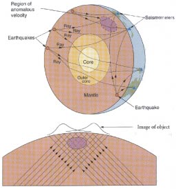
All high-resolution methods for determining Earth’s
interior structure are based on analyzing the propagation
of seismic waves generated by earthquakes
and explosions. These are elastic waves, in which
the restoring forces come from the resistance of materials
to deformation. In an infinite medium they are of
two types: compressional waves, of which
sound waves in air are the most familiar example,
and shear waves, which propagate only in
solids. Compressional and shear waves are called body
waves, because they propagate through the body
of the Earth.
Seismic waves travel at speeds of several kilometers per second in
the Earth, with the speed of compressional waves, Vp, being
about 1.7 times greater than that of shear waves, Vs. Seismic
wave speeds are different in different kinds of rocks, and in addition
increase with pressure (which is very nearly a function of depth alone)
and decrease with temperature.Through seismic wave speeds, we know of
Earth’s major vertical subdivisions and their approximate compositions:
-
the crust, the outer few tens
of kilometers, on which we live.
-
the 2900-km thick mantle, composed
of ultramafic rocks.
-
the liquid iron core (radius 3475
km), at whose center is the 1250-km radius solid inner
core.
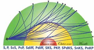
The boundaries between these major divisions
within the Earth produce many kinds of reflected and transmitted
seismic phases, some of which are shown at right, and
cause seismograms to be complicated. |
 |
Seismic wave speeds also vary horizontally, but this is a second-order
effect. For example, the crust is five to ten times thicker under continents
than under oceans. Beneath oceanic trenches the mantle is relatively cool
and wave speeds are high, and beneath oceanic spreading ridges the mantle
is hotter and wave speeds are lower.
Determining the seismic wave-speed distribution in
the mantle is the most powerful way to detect and map plumes. Since plumes
were first proposed by Morgan
[1971], seismologists have used many methods to look for anomalous
deep structures beneath hot spots, including plume heads, which might
be easier to detect, but so far they have had little success.
Predicted Effects
of Plumes on Seismic Structure
Direct thermal effect
– If thermal plumes exist in the mantle, they would have lower
seismic wave speeds than their surroundings. In the upper mantle, a
100 K temperature rise lowers Vp by about 1%, and Vs
by about 1.7%. In the deep mantle, this effect is several times weaker.
The minimum temperature anomalies proposed for plumes are about 200
K.
Indirect thermal effect
– Temperature variations would also cause variation in the depths
of polymorphic phase boundaries in the transition zone
between the upper and lower mantle. These are places where pressure
causes certain minerals to change their crystal structure, and these
changes are accompanied by jumps in density and seismic wave speed.
Two such zones in particular, at depths of about 410 and 650 km, are
global features and fairly easily detectable. A 100 K temperature rise
would depress the “410-km” discontinuity by about 8 km,
and raise the “650-km” discontinuity by about 5 km. (Both
of these numbers are based on the assumption that olivine is the main
mantle mineral, and are subject to significant uncertainty.) Thus a
high-temperature anomaly would produce negative and anomalies at 410
km and positive ones at 650 km. The depths to these phase changes can
also be measured directly using waves reflected from them (see
Receiver Functions, below).
Chemical effect
– If a plume has a different composition from the surrounding
mantle, this alone will cause a seismic wave-speed anomaly. The sign
and magnitude of the anomaly will depend on what minerals are involved,
but as a rule of thumb more buoyant materials have lower wave speeds.
Melting –
The presence of even a small amount of melt in a rock has a large effect
on its seismic-wave speeds. Partial melting may reflect either thermal
(high temperature) or chemical (low melting point) effects. The magnitude
of the effect on seismic wave speeds depends strongly on the geometric
form of the melt bodies. Thin films on grain boundaries have the largest
effect, and approximately spherical melt bodies have the smallest effect
[Goes et al., 2000].
Anisotropy –
Seismic wave speeds and other properties of rocks vary with direction,
and this can be as strong an effect as spatial heterogeneity. Most studies
of Earth structure ignore this effect, and their results probably are
biased by this oversimplification. Studies dealing explicitly with anisotropy
are becoming more common.
Anelasticity
– Many physical mechanisms remove energy from seismic waves and
convert it to heat, causing the waves to eventually die away. A side
effect of this process is to introduce a weak frequency dependence on
the wave speeds, which must be accounted for in studies of Earth structure.
Seismic Tomography
The travel time of a seismic
wave through the Earth gives an average of the wave speed along
the wave’s ray path (but see Bananas
& Doughnuts, below). If travel times are available
for enough ray paths, passing through all parts of a region in
many different directions, it is possible to un-scramble the times
to determine the three-dimensional wave-speed distribution. The
term tomography, borrowed from medicine, is given to
such seismic techniques. Seismic tomography is much more difficult
than X-ray tomography, because the ray paths are curved and initially
unknown, and in some cases the locations of the sources are poorly
known. |
|
Three seismic tomography techniques are particularly
useful in searching for plumes:
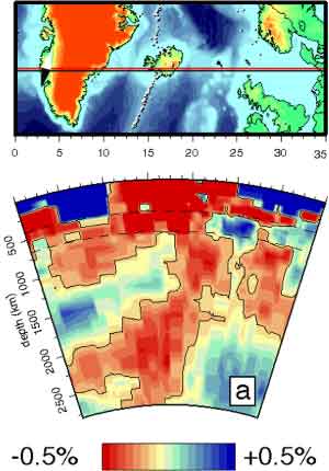
Cross section through a teleseismic tomography
model of Yellowstone [from Christiansen
et al., 2002]. |
Teleseismic Tomography
– In order to study the structure immediately under an area,
one can deploy an array of seismometers and record waves from distant
earthquakes (>~ 2,500 km away). Such waves arrive at angles within
about 30° of the vertical, so crossing rays sample the structure
down to depths comparable to the array aperture. The ray directions
are not isotropically distributed, however; and no ray paths are
ever close to horizontal. Consequently, compact structures tend
to be smeared vertically in images obtained by this technique [Keller
et al.,
2000]. This smearing is unfortunate, because it generates artifacts
that resemble the structures that are being sought. It is possible
to estimate quantitatively the severity of the smearing, however,
and if due attention is paid to this error source, teleseismic tomography
is the best technique available for studying the upper few hundred
kilometers of particular regions. An example of this kind of tomography,
applied to Iceland, is described by Foulger
et al.
[2001]. |
Whole-Mantle
Tomography – There
have now been thousands of seismometers deployed
globally for decades, and millions of travel-time
observations have accumulated and been used
to derive three-dimensional models of the whole
mantle. Some studies use enormous data sets
obtained from seismological bulletins such as
that of the International Seismological Centre,
but these data are subject to large and systematic
observational errors. Others use data measured
in more objective and consistent ways, usually
using digitally recorded seismograms. Most whole-mantle
models agree about the largest-scale anomalies
(thousands of kilometers in size), but for a
long time this was not so. The model that currently
has the best resolution at depths of a few hundred
kilometers, most critical for the search for
plumes, is described by Ritsema
et al.
[1999]. |
Cross section through a whole-mantle tomography
model through Yellowstone [courtesy of J.
Ritsema]. |
The resolution of these models is limited both by the
ray distributions and by the state of computer technology. The smallest
anomalies currently resolvable are 500 km or more in size. Furthermore,
ray paths fall far short of sampling the Earth uniformly. Both earthquakes
and seismometers are distributed irregularly over the Earth, and some
places within the Earth are sampled poorly or not at all e.g.,
the southern hemisphere, and particularly the Indian Ocean. The uneven
ray distribution also systematically distorts anomalies in the Earth.
As with teleseismic tomography, this distortion can be assessed quantitatively,
but not by the general reader unless considerable information on this
subject is given in the paper in question.
Surface-wave Tomography
– Tomographic methods can also be applied to surface waves,
low-frequency seismic waves that propagate in the crust and upper mantle
and owe their existence to the presence of the free surface. The depths
to which surface waves are sensitive depends on frequency, with low-frequency
waves "feeling" to greater depths and therefore propagating
at higher speeds. (Rule of thumb: Surface waves feel down to about a
quarter of their wavelength. They also propagate at about 4 km/s, so
this depth, in kilometers, is about 1/frequency (Hz).)
Because of the distribution of earthquakes and seismometers,
surface waves can often sample regions of the crust and upper mantle
that body waves do not. They are also expected to be highly sensitive
to plume heads, which are predicted to flatten out in the upper mantle,
producing low wave speed regions that extend for thousands of km [Anderson
et al., 1992]. Body-wave and surface-wave data are often combined
in whole-mantle tomography studies, such as that of Ritsema shown above.
Bananas
& Doughnuts – The statement above, that
travel times are averages along ray paths, is a simplification. In reality,
seismic waves “feel” the structure in a finite volume, and
in fact Dahlen et al. [2000] have recently shown that travel
times are most sensitive near a hollow surface around the ray, whose
shape reminds them of certain snack foods. Incorporation of this insight
into tomographic practice will significantly improve the quality of
three-dimensional Earth models, but only preliminary
results are, as yet, available.
Highly saturated cross section
of Iceland through the model of Bijwaard
& Spakman [1999].
Less saturated cross section, also of Iceland,
through the model of Ritsema
et al. [1999]. |
Caveat emptor!
Several aspects of graphical presentation may
make it difficult to interpret three-dimensional models in terms
of Earth structure and processes:
- A model typically includes a huge amount of information,
only a small fraction of which is shown, usually in the form
of maps at various depths or vertical cross sections. The
visual impression of the results given may be very sensitive
to the precise position of the section.
- Wave speeds are usually displayed with colors, blue representing
high wave speeds and red representing low ones. It is natural
to associate red colors with higher temperatures. However,
many factors affect the wave speed, including composition,
crystal orientation, mineralogy and phase (especially the
presence of melt). Red anomalies may not really be hot, nor
blue ones cold.
- The eye’s sensitivity to color varies greatly across
the spectrum, so inevitably some features are prominent while
other, equally strong ones, are nearly invisible. For example,
the transition from blue to yellow is much more noticeable
than that from orange to red.
- If the color scale saturates, anomalies may look the same
when they actually differ in strength by an order of magnitude.
For example, lower-mantle anomalies are much weaker than upper-mantle
ones, but this is obscured in figures where the color scale
saturates at the maximum lower-mantle anomaly [Anderson,
1999].
Because of these factors, the appearance of tomographic
images may be highly variable, depending on graphical design choices
made by seismologists. |
The Simple Direct
Approach
Because they have limited resolution and can distort anomalies in complicated
ways, tomographic results often are difficult to interpret. It would
be much better if seismic waves sampled precisely a region of interest,
and nothing else. Happily, nature occasionally arranges an experiment
for us in just this way. For example, the seismic phase ScS,
a shear wave reflected from the core-mantle boundary (CMB), when observed
close to the epicenter of an earthquake, has a nearly vertical ray path
through the entire mantle (Anderson & Kovach, 1964). Such
waves are ideally suited to looking for vertical plumes.
On April 26,1973, a magnitude 6.2 earthquake occurred in Hawaii, and
the records from seismometers on Oahu show an usually clear train of
multiple-ScS phases, reflected repeatedly between the Earth’s
surface and the CMB [Best et al., 1975]. These waves are sensitive
to structure in a vertical cylinder with a diameter of about 500 to
1000 km extending down to the CMB, and they show no indication of a
plume. The wave speed Vs in the upper and middle
mantle inferred from arrival times is higher than the average for the
southwestern Pacific [Katzman et al., 1998 Plate 3(b)], and
the propagation efficiency is also high (i.e., the waves are
little attenuated) [Sipkin & Jordan, 1979]. The location
of a possible plume in the lower mantle might be far enough from Hawaii
that these ScS waves would not sample it, but these observations
argue strongly against unusually high temperatures or extensive melting
in the upper mantle beneath Hawaii.
Receiver
Functions
When a compressional or shear seismic wave strikes a discontinuity
in the Earth, it generates reflected and transmitted waves of both types.
Because of this, waves from distant earthquakes passing through a layered
medium such as the crust or upper mantle generate complicated seismograms
containing many echoes. To interpret these records, seismologists process
them to generate simplified artificial waveforms, somewhat inscrutably
called receiver functions. These can be inverted to yield the
variation of Vs with depth, and they are particularly sensitive
to strong wave-speed discontinuities. Receiver functions are particularly
powerful for studying the depths to the Moho and the “410-km”
and “650-km” discontinuities, which may provide evidence
about crustal thickness and temperature at these depths [Du
et al., 2002].
One of the most detailed receiver-function
studies done to date took the form of a profile across the eastern
Snake River Plain, the suggested track of a mantle plume now beneath
Yellowstone, which lies at the northeastern end of the Plain [Dueker
& Sheehan, 1997]. The results illustrate the complexity
of structures revealed by receiver functions, and some of the
difficulties of interpreting them. Several “discontinuities”
are present, in addition to the major ones near 410 and 650 km.
Even these two major features are not continuous, and the 410-km
discontinuity appears to split in two near the left end of the
profile. The depths to the 410- and 650-km discontinuities are
expected to be negatively correlated if their topography results
from temperature variations, but actually they are weakly positively
correlated. The receiver functions thus provide no evidence of
elevated temperatures in this region. |
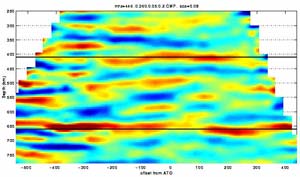
Vertical cross-section showing receiver functions
(mapped from the time domain to depth) computed for seismograms
recorded on a northwest-southeast profile across the eastern Snake
River Plain in southeastern Idaho, near the Yellowstone hot spot.
Colors indicate zones of rapid increase (red) and decrease (blue)
of with depth. Black horizontal lines: nominal depths of the 410-
and 650-km discontinuities. Figure from the
website of Ken Dueker, University of Wyoming. |
The
Base of the Mantle
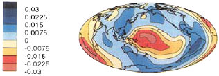
Base of the mantle according to the model of
Bhattacharyya et al. [1996]. |
The lowest few hundred kilometers of the Earth’s
mantle, just above the liquid-iron core, are much more heterogeneous
than the 2,000-km thick mantle region above. This basal boundary
layer, also known as D'' ("D double primed") was originally
detected in studies the travel times of seismic waves from deep
earthquakes [Julian & Sengupta, 1973] and has subsequently
been verified by results from many different kinds of investigations. |
Summary
The main methods for studying Earth structure in a way that is useful
in the search for plumes include seismic tomography, studying the transit
times and attenuation of individual waves that penetrate the volume
of interest, and the use of receiver functions to study topography on
the boundaries of the transition zone. Whereas downgoing slabs in subduction
zones and their effects on the transition zone have been easy to detect,
the same cannot be said about plumes, heads or tails, and promising
images often have not proved reproducible by later, more detailed studies.
It will be interesting to follow what the next decade brings.
News
& Discussion
A variety of plumes in
the mantle?
-
Anderson, D.L. and
Kovach, R.L., 1964, Attenuation in the mantle and
rigidity of the core from multiple reflected core
phases, Proc. Nat'l Acad. Sci., 51,
168-172.
-
Anderson, D.L.,
Are color cross sections really Rorschach tests?,
EOS Trans. AGU, 80, F719,
1999.
- Anderson, D.L., T. Tanimoto and Y.-S.
Zhang, Plate tectonics and hotspots: The third dimension,
Science, 256, 1645-1650,
1992.
- Best, W.J., L.R. Johnson and T.V. McEvilly,
ScS and the mantle beneath Hawaii, EOS
Fall Meeting Supplement, 1147, 1975.
- Bhattacharyya, J., G. Masters, and
P. Shearer, Global lateral variations of shear wave
attenuation in the upper mantle, J. geophys. Res.,
101, 22,273-22,289, 1996.
- Bijwaard,
H. and W. Spakman, Tomographic evidence for a narrow
whole mantle plume below Iceland, Earth Planet.
Sci. Lett., 166, 121-126.
-
Dahlen, F.A., S.-H.
Hung, and G. Nolet, Frechet kernels for finite-frequency
traveltimes - I. Theory, Geophys. J. Int.,
141, 157-174, 2000.
- Christiansen,
R.L., G.R. Foulger, and J.R. Evans, Upper mantle origin
of the Yellowstone hotspot, Bull. Geol. Soc. Am.,
114, 1245-1256, 2002.
-
Du,
Z., G.R. Foulger, B.R. Julian, R.M. Allen, G. Nolet,
W.J. Morgan, B.H. Bergsson, P. Erlendsson, S. Jakobsdottir,
S. Ragnarsson, R. Stefansson, and K. Vogfjord, Crustal
structure beneath western and eastern Iceland from
surface waves and receiver functions, Geophys.
J. Int., 149, 349-363, 2002.
-
Dueker, K.G., and
A.F. Sheehan, Mantle discontinuity structure from
midpoint stacks of converted P to S
waves across the Yellowstone hotspot track, J.
geophys. Res., 102, 8313-8327,
1997.
-
Foulger,
G.R., M.J. Pritchard, B.R. Julian, J.R. Evans, R.M.
Allen, G. Nolet, W.J. Morgan, B.H. Bergsson, P.
Erlendsson, S. Jakobsdottir, S. Ragnarsson, R. Stefansson,
and K. Vogfjord, Seismic tomography shows that upwelling
beneath Iceland is confined to the upper mantle,
Geophys. J. Int., 146,
504-530, 2001.
-
Goes, S., R. Govers,
and P. Vacher, Shallow mantle temperatures under
Europe from P and S wave tomography, J. geophys.
Res., 105, 11,153-11,169,
2000.
-
Julian, B.R., and
M.K. Sengupta, Seismic travel time evidence for
lateral inhomogeneity in the deep mantle, Nature,
242, 443-447, 1973.
- Katzman, R., L. Zhao, and T.H. Jordan,
High-resolution, two-dimensional vertical tomography
of the central Pacific mantle using ScS reverberations
and frequency-dependent travel times, J. geophys.
Res., 103, 17,933-17,971, 1998.
-
-
-
-
Sipkin, S.A., and
T.H. Jordan, Lateral heterogeneity of the upper
mantle determined from the travel times of ScS,
J. geophys. Res., 80,
1474-1484, 1975.
- Sipkin, S.A., and T.H. Jordan, Frequency
dependence of QScS, Bull. seismol. Soc.
Am., 69, 1055-1079, 1979.
last
updated 31st December, 2006 |
 MECHANISMS